Calculating Impervious Surface Area

Introduction

In this lab we will segment and classify aerial imagery by land use in order to calculate the amount of impervious surface area per parcel of land. Some municipalities will charge home/land owners extra fees based on the amount of impervious surface area on their land because too high an amount of it can cause flooding issues.

Methods

Segment the Imagery

We first started by downloading the dataset from the ArcGIS tutorial website. The lab begins by extracting the spectral bands in order for us to better distinguish some of the urban features, like concrete, from natural features, such as vegetation. The extracted bands are 4, 1, and 3 which respectively emphasize vegetation, man-made objects, and water. Figure 1 shows the image after band extraction.

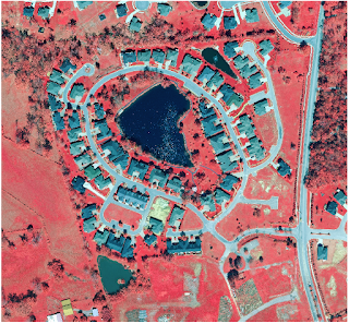Figure 1: Extract Bands function used

We utilize the classification wizard is used throughout much of this lab to help us classify different parts of the image. However, we leave the image segmentation alone because the next step is to create our own segmented image.  The segmented image will look like Figure 2.

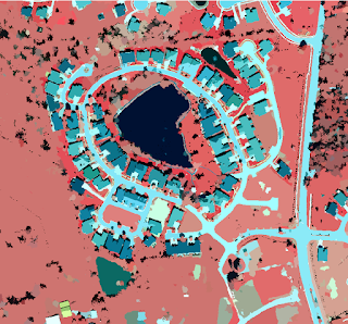Figure 2: Spectral Band Extraction on the Segmented Image

Classify the Imagery

After the segmented image has been created, we can begin to classify the image. We classified this image into the two main classes of pervious and impervious, within these two classes we have smaller classes to represent types of land cover. We create training samples to classify the imagery. Training samples are polygons that represent specific areas of different land cover type. We created seven groups of training samples for our image. These groups were grey roofs, roads, driveways, bare earth, grass, water and shadows. Figure 3 below shows our classified image with the colors we have chosen for each training class.

Figure 3: Classified Image

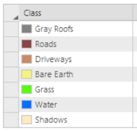Figure 4: Training Samples

After classifying the image we then reclassify any errors in classification. If the data shows misclassifications we can go back and change them manually. I did not change any of the classifications in my data set. The resulting image is shown in Figure 5, this image shows only pervious and impervious surfaces.

Figure 5: Pervious and Impervious Surfaces

 Now we can begin to calculate surface area. We start by creating accuracy points, we made 100 points. These are shown in Figure 6 and 7.

Figure 6: Accuracy Points

Figure 7: Accuracy Points Attribute Table

In the attribute table we must manually go in and change ground truth to 20 or 40 depending on the location of the point with 20 being pervious and 40 being impervious. Next, we computed a confusion matrix and tabulated the area. A confusion matrix will determine the accuracy of the classified and GrndTruth attributes. The confusion matrix results are shown in Figure 8 below.

Figure 8: Confusion Matrix

Tabulating the area will show the pervious and impervious area within each parcel, this is shown in Figure 9 below.

Figure 9: Tabulated Area

Now that we have calculated the impervious surface are we need to symbolize the parcels. We chose a yellow to red gradient to symbolize surface area. The symbolized parcels are pictured in Figure 10 below.

Figure 10: Symbolized Parcels

Conclusion

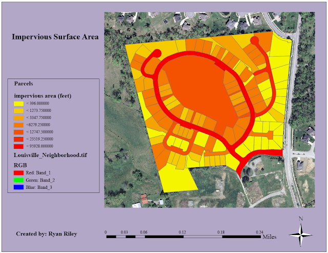Figure 11: Map of Impervious Area

In the map we are able to analyze the amount of impervious surface area per each individual land parcel. Local governments and civil institutions can utilize this data to determine storm water bills. We can determine how much impervious surface are each parcel has by comparing the color on the map with the corresponding color in the legend. As we can see the road contains the most impervious area of all the parcels which is what we had expected.